Time-Varying Confounding: A Summary of Key Ideas and Frequently Asked Questions

A Hypothetical Example with Publicly Subsidized Housing as the Exposure

To facilitate our discussion of time-varying confounding, we present a hypothetical example in which we are interested in studying the effects of public housing subsidies over time on child cognition (Figure 1). In this example, we have measures of receipt of a subsidy for public housing and income at both baseline and follow-up as well as a measure of child cognition at follow-up. The time-varying exposure we wish to evaluate is receipt of public housing subsidies. We hypothesize that both baseline and follow-up public housing subsidies influence child cognition at follow-up. Furthermore, we consider income a potential time-varying confounder. That is, income at baseline and income at follow-up influence both access to public housing subsidies as well as child cognition. Lastly, and critically because time-varying confounders affected by prior exposure are difficult to address, we postulate that public housing subsidies at baseline influence income at follow-up.

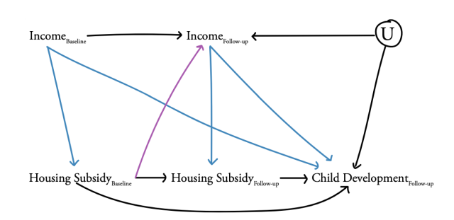
Note: Here we provide a hypothetical, simplified example depicting the problem of time-varying confounding (e.g., we omit several possibly pathways for simplicity). The light blue lines depict confounding from income that occurs at both baseline and follow-up (i.e., time-varying confounding). The purple line highlights the problematic pathway in which the income at follow-up is affected by prior exposure to housing subsidies, thereby inducing the potential for treatment-confounder feedback. In a traditional regression framework, controlling for Income_Follow-up addresses confounding of the Housing Subsidy_Follow-up — Child Cognition_Follow-up relationship but also controls away part of the pathway of interest from Housing Subsidy_Baseline to Child Cognition_Follow-up. U is a set of unmeasured factor(s) that influence income at follow-up and child cognition at follow-up. U helps demonstrate why income at follow-up is a collider variable. Conditioning on income at follow-up induces noncausal associations between baseline receipt of housing subsidies and U, thereby potentially opening biasing pathways since U affects child cognition.

Time-Varying Confounding

Confounding occurs when there are shared causes of the exposure and the outcome. Note, from here on out we will use the term “exposure” or “exposures” to interchangeably represent treatments, interventions, policies, programs, or conditions an individual might be exposed to. This shared cause is an example of a confounder, because it influences both the exposure and the outcome (for more on confounding, see our blog post and method note on confounder versus instrumental variable designs). This “mixing” of effects distorts the primary association of interest between the exposure and the outcome (the effect of the exposure on the outcome is mixed with the effect of the confounder on the outcome). In our example, the confounding effects of income at baseline and at follow-up are represented in blue. Time-varying confounding occurs when the value of the confounder changes over time and thus its influence on the outcome of interest also changes over time. In this example, income changes from baseline to follow-up and income at both time points influence child cognition (i.e., the two sets of blue arrows emanating from income at baseline and follow-up, respectively).

Time-Varying Confounding and Treatment Confounder Feedback

Time-varying confounders are especially problematic when they are affected by past exposures – e.g., consider the purple line in Figure 1 where baseline receipt of public housing subsidies affects later income at follow-up. The purple pathway indicates a conundrum known as “treatment-confounder feedback” or exposure-confounder feedback.¹ This feedback has been described as treatment induced, intermediate, post-treatment, time-dependent or time-varying confounding.² Note that time-varying confounding can occur without treatment-confounder feedback.¹ However, when there are time-varying confounders and treatment-confounder feedback, we need special methods to control for the time-varying confounding while addressing the treatment-confounder feedback because conventional methods such as regression, stratification, or matching estimators are biased.^3-4

To understand this conundrum further, again consider our hypothetical example. Housing subsidies may provide parents with stable housing that enables them to pursue additional education and improved work opportunities. Those enhanced work and income opportunities attainable by virtue of stable housing may, in turn, affect both future eligibility for housing subsidies and children’s long-term cognition. In other words, there is feedback because prior receipt of public housing subsidies influences future income and that future income influences later receipt of public housing subsidies and child cognition. Not accounting for this feedback may lead to incorrect conclusions about the effects we care about, especially as the number of time points in our study grows. We need to think about how to handle, or separate, this treatment-confounder feedback when we ultimately focus on unpacking our effect of interest (i.e., mainly the effect of public housing subsidies over time on child cognition).

Why do conventional regression methods fail?

Conventional regression, stratification, or matching estimators that condition on (e.g., adjust for) time-varying confounders affected by prior exposure may result in biased effect estimates for two reasons.⁵ In this discussion, we rely on the concepts of backdoor paths and collider variables in causal diagrams. For more information on these topics, refer to Pearl (2009)⁶ and Glymour and Greenland (2008).⁷

Initial intuition might be that, to control for confounding by income, we should condition on both income at baseline and income at follow-up. By conditioning on income at baseline, we block potential “nuisance” backdoor paths between public housing subsidies and child cognition that would otherwise confound estimates of the effect of interest. However, the problem arises when we condition on income at follow-up. One of the core rules for estimating causal effects of an exposure is not to condition on anything that is on a causal pathway connecting the exposure and the outcome of interest. When we condition on follow-up income, we block the part of the effect of the baseline public housing subsidy receipt that acts through income at follow-up. This pathway represents part of the causal effect of housing subsidy at baseline on child cognition at follow-up, so the adjusted estimate is biased from the total effect of subsidy receipt. This issue has also been referred to as over-adjustment bias and overcontrol.^4,8,9

Another bias can occur when controlling for a covariate that is influenced by our exposure if the covariate is what is called a “collider.” Conditioning on a collider variable can induce noncausal associations—for example between an exposure at baseline and an end-of-study outcome. In our example, when we condition on income at follow-up, which is affected by both prior public housing subsidies and other – likely unmeasured – factors such as “U,” income at follow-up is the “collider variable.” Conditioning on income at follow-up induces noncausal associations between baseline receipt of housing subsidies and U, thereby potentially opening biasing pathways since U affects child cognition. This issue is also known as “collider-stratification bias.”¹⁰

How can we control for time-varying confounding?

Several technical papers have been published in the last 35 years describing how to appropriately handle time-varying confounding and measure the causal effects of time-varying exposures. We think of these methods as boiling down to the following approaches:

Breaking the link between the confounders and the exposure:

Methods such as inverse probability of exposure-weighting (IPEW) involve modeling the exposure at each time point based on the previous values of confounders and the exposure. This ‘exposure model’ is used to estimate a set of time-varying weights, which are the inverse of the probability that each individual received the exposure they actually received at each time-period, conditional on their own past history up to that time period. When we apply these weights to the original data set (creating what is sometimes called a ‘pseudo-population’), the exposure and confounder history are unrelated. Then, the effect of the exposure at each time period on the outcome is modeled using the reweighted data set. IPEW approaches assume we have correctly specified the exposure model (i.e., it includes all the variables that need to be adjusted and assumes the correct shapes for the relationships between these variables and the exposure).

Breaking the link between the confounders and the outcome:

Some methods focus on iteratively accounting for the confounders over time when modeling the outcome. For example, G-computation methods sequentially model the confounder values at each time point to predict how time-varying confounders would have evolved if we had intervened to set the exposure to a particular sequence (e.g., “always receive public housing subsidies”). These hypothetical trajectories of the confounders are then used instead of actual confounder values when estimating the effects of the exposure sequence on the outcome. Another approach, G-estimation of structural nested mean (SNM) models, focuses on choosing coefficients that fulfill the assumption of conditional exchangeability across time. That is the assumption that, conditional on the covariates, each person’s exposure is unrelated to the potential outcome they would have under any possible exposure (conditional on covariates). Estimation of SNMs can be based on grid-searching for a causal effect estimate such that this assumption is fulfilled. Both G-computation and G-estimation require assumptions about correct specification of the outcome model.

Breaking the link between confounders and both exposure and outcomes:

Doubly robust methods combine approaches to break the link between the confounders and the exposure and break the link between the confounders and the outcome. If either the model for exposure or the model for the outcome is correctly specified, the estimate is unbiased. Doubly robust methods are appealing because they offer two chances to specify the model correctly.

For a more in-depth review of different methods for handling time-varying confounding in recent literature, we recommend the following references.^3,9,11-13

How are studies using methods to control for time-varying confounding?

Although methods to address time-varying confounding have existed for over three decades,¹⁴ uptake of these methods has been slow and limited in substantive scope. Slow uptake may be in part because the statistical tools were challenging to implement and required large sample sizes. In recent years, the methods have become easier to apply, and innovations such as Targeted Maximum Likelihood Estimation have improved statistical efficiency even for moderate sample sizes. Relatively accessible summaries of these methods have recently been published1 that build on more technical earlier work.^14-15 Newer methods advancing on these ideas have improved flexibility and statistical power and reduced sensitivity of results to violations of some assumptions required by the methods.^2,16-18

A recent study¹² provided a systematic review of studies published in any discipline between 2000 to 2016 that used or discussed methods for time-varying confounding. The study found 542 studies during the period: in 2000 there were just 2 studies that met their criteria and by 2016 this had risen to only 112. A large fraction of the applications of methods for time-varying confounding were focused on only a handful of areas. For example, of the 432 studies between 2009- 2016, over 60% of articles were applications in HIV (30.6%), cardiopulmonary (13.2%), kidney disease (11.8%), and mental health (10.0%) research. Lastly, the study found that IPEW was the most commonly utilized method to address time-varying confounding, even if IPEW may not always be the most robust option.^17-19

Time-varying confounding creates the potential for bias in estimating the health effects of exposures that change over time. Specialized methods for handling time-varying confounding can help reduce this bias. The slow adoption of methods for time-varying confounding is a loss for the health relevance of our research because many exposures would have little effect in short, small doses, but may have large and important effects after sustained exposure. For some exposures of special interest to health equity, for example income, stability itself may be an important feature, i.e., we should be evaluating how volatility in income influences health. Such analyses will almost certainly require methods to address time-varying confounding.

The method to control time-varying confounding that researchers ultimately choose should match the study's characteristics (i.e., the model needs to be correctly specified) and be the most robust option available (i.e., likely to provide accurate and precise estimates even if the assumptions are slightly violated). To the extent that simulation-based evidence is available, such studies can help inform researchers regarding which methods are most accurate and precise and for which settings. Doubly robust methods can offer gains in precision over alternative methods and some doubly robust methods allow researchers to flexibly incorporate a wide range of machine learning algorithms while maintaining valid statistical inferences.^17-19

The uptake of methods for controlling time-varying confounding may have been slowed by the complexity of the methods and the availability of software to implement them. Fortunately, more recent research has provided examples of how to implement G-estimation methods for handling time-varying confounding in the open-source platform R.^2,11 Given the rapidly expanding suite of methods and user-friendly tools, we anticipate that future population health and health equity researchers will be better equipped to address important questions about time-varying exposures.

1. Hernán MA, Robins JM (2020). Causal Inference: What If. Boca Raton: Chapman & Hall/CRC.
2. Loh, W. W., Moerkerke, B., Loeys, T., Poppe, L., Crombez, G., & Vansteelandt, S. (2020). Estimation of controlled direct effects in longitudinal mediation analyses with latent variables in randomized studies. Multivariate Behavioral Research, 55(5), 763-785.
3. Naimi, A. I., Cole, S. R., & Kennedy, E. H. (2017). An introduction to g methods. International Journal of Epidemiology, 46(2), 756-762.
4. Mansournia, M. A., Etminan, M., Danaei, G., Kaufman, J. S., & Collins, G. (2017). Handling time-varying confounding in observational research. BMJ, 359:j4587.
5. Daniel, R. M., De Stavola, B. L., & Cousens, S. N. (2011). Gformula: Estimating causal effects in the presence of time-varying confounding or mediation using the g-computation formula. The Stata Journal, 11(4), 479-517.
6. Pearl, J. (2009). Causality. Cambridge University Press.
7. Glymour, M. M., & Greenland, S. (2008). Causal diagrams. Modern Epidemiology, 3rd edn (eds K.J. Rothman,S. Greenland, and T.L. Lash), Lippincott Williams & Wilkins, Philadelphia, Chapter 12, 183- 209.
8. Schisterman, E. F., Cole, S. R., & Platt, R. W. (2009). Overadjustment bias and unnecessary adjustment in epidemiologic studies. Epidemiology, 20(4), 488.
9. Wodtke, G. T. (2020). Regression-based adjustment for time-varying confounders. Sociological Methods & Research, 49(4), 906-946.
10. Hernán, M. A., Hernández-Díaz, S., & Robins, J. M. (2004). A structural approach to selection bias. Epidemiology, 615-625.
11. Acharya, A., Blackwell, M., & Sen, M. (2016). Explaining causal findings without bias: Detecting and assessing direct effects. American Political Science Review, 110(3), 512-529.
12. Clare, P. J., Dobbins, T. A., & Mattick, R. P. (2019). Causal models adjusting for time-varying confounding—a systematic review of the literature. International Journal of Epidemiology, 48(1), 254-265.
13. Vansteelandt, S., & Sjolander, A. (2016). Revisiting g-estimation of the effect of a time-varying exposure subject to time-varying confounding. Epidemiologic Methods, 5(1), 37-56.
14. Robins, J. (1986). A new approach to causal inference in mortality studies with a sustained exposure period—application to control of the healthy worker survivor effect. Mathematical Modelling, 7(9-12), 1393-1512.
15. Robins, J. M. (1999). Association, causation, and marginal structural models. Synthese, 151-179.
16. Bang, H., & Robins, J. M. (2005). Doubly robust estimation in missing data and causal inference models. Biometrics, 61(4), 962-973.
17. Petersen, M., Schwab, J., Gruber, S., Blaser, N., Schomaker, M., & van der Laan, M. (2014). Targeted maximum likelihood estimation for dynamic and static longitudinal marginal structural working models. Journal of Causal Inference, 2(2), 147-185.
18. van der Laan, M.J., & Rose, S. (2011). Targeted Learning: Prediction and Causal Inference for Observational and Experimental Data. New York: Springer-Verlag.
19. Wyss, R., Schneeweiss, S., Van Der Laan, M., Lendle, S. D., Ju, C., & Franklin, J. M. (2018). Using super learner prediction modeling to improve high-dimensional propensity score estimation. Epidemiology, 29(1), 96-106.

The E4A Methods Lab was developed to address common methods questions or challenges in Culture of Health research. Our goals are to strengthen the research of E4A grantees and the larger community of population health researchers, to help prospective grantees recognize compelling research opportunities, and to stimulate cross-disciplinary conversation and appreciation across the community of population health researchers.